Neural Network – IRIS data Classification Model, Dr. Arunachalam Rajagopal
Neural Network – IRIS data Classification Model
by Dr. Arunachalam Rajagopal
Artificial Neural Network (ANN):
A typical artificial neural network is shown in Figure 1. ANN is a sub-domain of artificial intelligence, AI. ANNs attempt to
imitate the behaviour of human brain for problem solving by creating an
abstract model. ANN models which are basically non-linear in nature could
abstract and represent any non-linear function.
Activation function: introduces the non-linear characteristics into the
neural network. The activation function is selected based on the type of data
to be modeled. The often used activation
functions are:
Rectified Linear Unit (ReLu)
Logistic function
Hyperbolic tangent (tanh)
Figure 1 Artificial Neural Network
Example Demo: Neural
Network
The iris data set has been made use of for demonstrating the development
of neural network classification model. The Figure 2 shows the three flowers in the iris family which are Setosa, Versicolor, and Virginica. IRIS dataset comprises of 150 samples:
50 Setosa
50 Versicolor
50 Virginica
The variables in the data set are: Sepal Length, Sepal Width, Petal Length,
Petal Width
Figure 2 iris flowers (setosa, versicolor, virginica)
AI and Machine Learning:
Artificial Intelligence (AI)
Machine Learning
Deep Learning
Artificial Neural Networks (ANNs): ANNs are part of Machine Learning and
the ANNs comprises of:
Input Layer
Hidden Layer
Output Layer
Weights and biases
Activation function, f(z)
ANNs model with Activation function:
z = Sum(weights * inputs + bias)
output signal = f(z), where ‘f’ is the activation function.
Activation function, is applied on the weighted sum of inputs plus bias. The Figure 3 depicts a typical ANN with activation function indication.
Figure 3 ANN model showing the activation function
Neural Network for
iris data classification model:
> irisdata<-read.csv("iris.csv", sep=",",
header=T,row.names="id")
> head(irisdata)
tail(irisdata)
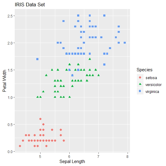
The Figure 4 shows a scatter between Sepal Length and Petal Width of the three flowers in the iris family. In fact, six scatter graphs could be drawn with four regressor variables (4c2=6).
> #Scatter plot: Sepal.Length versus Petal.Width
> library(ggplot2)
> ggplot(irisdata, aes(x=Sepal.Length, y=Petal.Width)) +
+ geom_point(aes(colour=Species,
shape=Species), size=2) +
+ ylab("Petal Width") +
+ xlab("Sepal Length")
+
+ ggtitle("IRIS Data
Set")
Figure 4 iris scatter with ggplot
> #data preparation for neural network model
> irisdf <- data.frame(SpCode = irisdata$SpCode, SpLength =
irisdata$Sepal.Length, SpWidth = irisdata$Sepal.Width, PtLength =
irisdata$Petal.Length, PtWidth = irisdata$Petal.Width)
> head(irisdf)
> tail(irisdf)
> #data normallization: minmax method
> maxval <- apply(irisdf[,1:5], 2, max)
> minval <- apply(irisdf[,1:5], 2, min)
> scaledf <-
data.frame(scale(irisdf[,c(1:5)],center=minval,scale=(maxval-minval)))
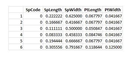
> head(scaledf)
> tail(scaledf)
> #train and test data by indexing
> index<-sample(2, nrow(scaledf), replace=T, prob=c(0.7,0.3))
> table(index)
index
1 2
113 37
> traindata<-scaledf[index==1,]
> testdata<-scaledf[index==2,c(2:5)]
> nrow(traindata)
[1] 113
> nrow(testdata)
[1] 37
> #neural network model for iris classification
> library(neuralnet)
> nnmodel<-neuralnet(SpCode~SpLength+SpWidth+PtLength+PtWidth,
data=traindata, hidden = 4, threshold=0.01)
> plot(nnmodel)
Figure 6 neuralnet model for iris classification
The Figure 6 shows the neural network diagram for the iris flower classification model. The neural network model has been developed with neuralnet package from R-CRAN.
> class(nnmodel)
[1] "nn"
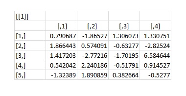
> nnmodel$weights[[1]][1]
#weights input layer to hidden layer
> nnmodel$weights[[1]][2]
> #neural network model fit
> fitval<-nnmodel$net.result[[1]][,1]
>
levelfitval<-fitval*(max(irisdata$SpCode)-min(irisdata$SpCode))+min(irisdata$SpCode)
> levelfitval<-as.integer(round(levelfitval,0))
> levelfitval
[1] 1 1 1 1 1 1 1 1 1 1 1 1 1 1 1
1 1 1 1 1 1 1 1 1 1 1 1 1 1 1 1 1 1 1 1 1 1
[38] 1 2 2 2 2 2 2 2 2 2 2 2 2 2 2
2 2 2 2 2 2 2 2 2 2 2 2 2 3 2 2 2 2 2 2 2 2
[75] 2 2 3 3 3 3 3 3 3 3 3 3 3 3 3
3 3 3 3 3 3 3 3 3 3 2 3 3 3 3 3 3 3 3 3 3 3
[112] 3 3
> actual.train<-irisdata$SpCode[index==1]
> actual.train
[1] 1 1 1 1 1 1 1 1 1 1 1 1 1 1 1
1 1 1 1 1 1 1 1 1 1 1 1 1 1 1 1 1 1 1 1 1 1
[38] 1 2 2 2 2 2 2 2 2 2 2 2 2 2 2
2 2 2 2 2 2 2 2 2 2 2 2 2 2 2 2 2 2 2 2 2 2
[75] 2 2 3 3 3 3 3 3 3 3 3 3 3 3 3
3 3 3 3 3 3 3 3 3 3 3 3 3 3 3 3 3 3 3 3 3 3
[112] 3 3
> tb1<-table(actual.train,levelfitval)
> tb1
levelfitval
actual.train 1 2 3
1 38 0 0
2 0 37 1
3 0
1 36
> accuracy1<-sum(diag(tb1))/sum(tb1)
> accuracy1 #classification
accuracy
[1] 0.9823009
> error1 <- 1-sum(diag(tb1))/sum(tb1)
> error1 #proportion of
misclassification
[1] 0.01769912
> #neural network testing, prediction and evaluation
> fpre<-compute(nnmodel,testdata)
> predval<-fpre$net.result[,1]
>
levelpredval<-predval*(max(irisdata$SpCode)-min(irisdata$SpCode))+min(irisdata$SpCode)
> levelpredval<-as.integer(round(levelpredval,0))
> levelpredval
[1] 1 1 1 1 1 1 1 1 1 1 1 1 2 2 2
2 2 2 2 2 2 2 2 2 3 3 3 3 3 3 2 3 3 3 3 3 3
> actual.test<-irisdata$SpCode[index==2]
> actual.test
[1] 1 1 1 1 1 1 1 1 1 1 1 1 2 2 2
2 2 2 2 2 2 2 2 2 3 3 3 3 3 3 3 3 3 3 3 3 3
> tb2<-table(actual.test,levelpredval)
> tb2
levelpredval
actual.test 1 2 3
1 12 0 0
2 0 12 0
3 0 1 12
> accuracy2 <- sum(diag(tb2))/sum(tb2)
> accuracy2 #classification
accuracy
[1] 0.972973
> error2 <- 1-sum(diag(tb2))/sum(tb2)
> error2 #proportion of
misclassification
[1] 0.02702703
> #Jai Hind
> #StayHome
> #StayClean
Neural Network IRIS classification model with neuralnet package:
Neural Network IRIS classification model with neuralnet package:
Reference:
1. R-CRAN website: https://cran.r-project.org/
2. Kabacoff R.I. (2011), "R in Action: Data analysis and graphics with R", Manning Publishing Co., Shelter Island, NY.
Author can be reached at: arg1962@gmail.com 94883617261. R-CRAN website: https://cran.r-project.org/
2. Kabacoff R.I. (2011), "R in Action: Data analysis and graphics with R", Manning Publishing Co., Shelter Island, NY.


Comments
Post a Comment